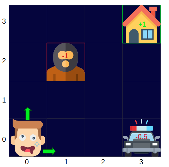
Our totally wasted grid world agent calls us and asks if we can safely navigate him home. We use the WhatsApp location sharing feature to determine the agent location. Our goal is to message the agent a policy plan which he can use to find his way back home. Like every drunk guy, the agent does noisy movements: he follows our instructions only in 80% of the time. In 10% of the time, he stumbles WEST instead of NORTH and in the other 10%, he stumbles EAST instead of NORTH. Similar behavior occurs for the other instructions. If he stumbles against a wall, he enters the current grid cell again. He gets more tired of every further step he takes. If the police catch him, he has to pay a fee and is afterward much more tired. On the way back home it could happen, that he gets some troubles with the “hombre malo”, and in his condition, he is not prepared for such situations. He can only rest if he comes home or meets the “hombre malo”. We want to navigate him as optimal as possible.
Markov Decision Process
Because of the noisy movement, we call our problem a non-deterministic search problem. We have to do 3 things to guide our agent safely home: First, we need a simulation of the agent and the grid world. Then we apply a Markov Decision Process (MDP) on this simulation to create an optimal policy plan for our agent which we will finally send via WhatsApp to him. An MDP is defined by a set of states \(s \in S\). This set \(S\) contains every possible state of the grid world. Our simulated agent can choose an action \(a\) from a set of actions \(A\) which changes the state \(s\) of the grid world. In our scenario he can choose the actions \( A = \{NORTH, EAST, SOUTH, WEST\}\). A transition function \(T(s,a,s’)\) yields the probability that \(a\) from \(s\) leads to \(s’\). A reward function \(R(s,a,s’)\) rewards every action \(a\) taken from \(s\) to \(s’\). In our case, we use a negative reward of \(-0.1\) which is also referred to \(\textit{living penalty}\) (every step hurts). We name the initial state of the agent \(s_{init}\) and every state which leads to an end of the simulation terminal state. There are 2 terminal states in our grid world. One with a negative reward of \(-1\) in \((1,2)\) and one with a positive reward of \(1\) in \((3,3)\).
Solving Markov Decision Processes
Our goal is to guide our agent from the initial state \(s_{init}\) to the terminal state \(s_{home}\). To make sure that our agent does not arrive too tired at home, we should always try to guide the agent to the nearest grid cell with the highest expected reward of \(V^{*}(s)\). The expected reward tells us how tired the agent will be in the terminal state. The optimal expected reward is marked with a *. To calculate the optimal expected reward \(V_{k+1}^*(s)\) for every state iteratively, we use the Bellman equation:
\(V^*_{k+1}(s) = \max_{a} Q^{*}(s,a)\) \(Q^{*}(s,a) =\sum_{s’}^{}T(s,a,s’)[R(s,a,s’) + \gamma V^{*}_{k}(s’)]\\\) \(V_{k+1}^*(s) = \max_{a} \sum_{s’}^{}T(s,a,s’)[R(s,a,s’) + \gamma V_{k}^{*}(s’)]\\\)\(Q^{*}(s, a)\) is the expected reward starting out having taken action \(a\) from state \(s\) and thereafter acting optimally. To calculate the expected rewards \(V^{*}_{k+1}(s)\), we set for every state \(s\) the optimal expected reward \(V_{0}^{*}(s) = 0\) and use the equation.
As soon as our calculations convergent for every state, we can extract an optimal policy \(\pi^{*}(s)\) out of it. An optimal policy \(\pi^(s)\) tells us the optimal action for a given state \(s\). To calculate the optimal policy \(\pi^{*}(s)\) for a given state \(s\), we use:
\(\pi^{*}(s) \leftarrow arg\max_{a} \sum_{s’}T(s,a,s’)[R(s,a,s’) + \gamma V_k^{*}(s’)]\)After we calculated the optimal policy \(\pi^{*}(s)\) we draw a map of the grid world and put in every cell an arrow which shows the direction of the optimal way. Afterward, we send this plan to our agent.
This whole procedure is called offline planning because we know all details of the MDP. But what if we don’t know the exact probability distribution of our agent stumbling behavior and how tired he gets every step? In this case we don’t know the reward function \(R(s,a,s’)\) and the transition function \(T(s,a,s’)\)? We call this situation online planning. In this case, we have to learn the missing details by making a lot of test runs with our simulated agent before we can tell the agent an approximately optimal policy \(\pi^*\). This is called reinforcement learning.
Reinforcement Learning
One day later our drunk agent calls us again and he is actually in the same state ;) as the last time. This time he is so wasted that he even can not calculate the reward function \(R(s,a,s’)\) and the transition function \(T(s,a,s’)\). Because of the unknown probabilities and reward function, the old policy is outdated. So the only way to get an approximately optimal policy \(\pi^{*}\) is to do online planning which is also referred to reinforcement learning. So this time we have to run multiple episodes in our simulation to estimate the reward function \(R(s,a,s’)\) and the transition function \(T(s,a,s’)\). Each episode is a run from the initial state of the agent to one of the terminate states. Our old approach of calculating \(\phi^{*}\) would take too long and it doesn’t convergent smoothly in the case of online training. A better approach is to do Q-Learning:
Q-Learning is a sample-based Q-value iteration To calculate the unknown transition function \(T(s, a, s’)\) we empirically calculate the probability distribution of the transition function.
This time we choose our policy based on the q-values of each state and update the \(Q(s, a)\) on the fly. The problem with this policy is, that it exploits always the best \(Q(s, a)\) which is probably not the optimal policy. To find better policies, we introduce a randomization/exploration factor to our policy. This forces the agent to follow sometimes a random instruction from us which leads to a better policy \(\pi^{*}\). This approach is referred to as \(\epsilon\)-greedy learning. After our \(Q(s, a)\) calculations converging, we can send the optimal policy to our agent.
Till now, our agent was lucky and he lived in a stationary grid world (all objects besides the agent are static). But as soon as the other objects start moving the grid world gets more complex and the number of states in the set \(S\) grows enormously. This could lead to a situation where it is not possible to calculate all the \(Q(s, a)\) anymore. In such situations, we have to approximate the \(Q(s, a)\) function. One way to approximate \(Q(s,a)\) functions is to use deep reinforcement learning.
References & Sources
- Haili Song, C-C Liu, Jacques Lawarrée, and Robert W Dahlgren. Optimal electricity supply bidding by Markov decision process.IEEE transactions on power systems, 15(2):618–624, 2000.
- Leslie Pack Kaelbling, Michael L Littman, and Andrew W Moore. Reinforcement learning: A survey.Journal of artificial intelligence research, 4:237–285, 1996.
- Christopher JCH Watkins and Peter Dayan. Q-learning.Machine learning, 8(3-4):279–292, 1992.
- Drunk guy image from flaticon.com
- Hombre malo image from flaticon.com
- Home image from flaticon.com
- Police image from flaticon.com