Around five years ago, Amazon released its smart assistant named Amazon Alexa. She has gained a lot of popularity among voice assistants. Most users use her to play music and search the internet for information. But these are just fun tasks. Alexa can help you with more of the daily tasks and make your life easier.
Amazon Alexa tries to be your assistant, but someone who reacts to commands doesn’t show any interpersonal relationship. This type of connection is essential for an assistant job – it builds respect and lets us see assistants like ‘individuals.’ This is one goal that AI developers want to achieve: Artificial Intelligence that is human-like. In this blog post, I want to discuss one possibility of achieving this goal.
Building an Interpersonal Relationship with Storytelling
A while ago, I read “Story” by Robert McKee. This book inspired me to think about human-like AI development a little bit differently.
Robert McKee describes in his books that a story is a metaphor for life – stories awaken feelings. When we watch good movies, we try to adopt the personal perspective of the movie characters. This leads to an ever-stronger bond with the characters in the course of the story.
This is exactly something that we want to achieve for our users and the virtual assistants. The field of storytelling reminds us that there is no way to love or hate a person if you have not heard that person’s story; that’s why our virtual assistant needs to have a backstory. As shown in the movie example, it makes no difference whether the person is real or not.
Often, a connection with movie characters arises when they make decisions in stressful situations. The real genius of a person manifests itself in the choices they make under pressure. The higher the pressure, the more the decision reflects the innermost nature of the figure. Stressful situations often appear for virtual assistants, such as when users ask for unanswerable questions. In this situation, ordinary virtual assistants answer with standard answers like, “I don’t understand,” or “I can’t help you.” In this case, the real character of the virtual assistant is revealed. AI developers have to avoid such standard answers, and instead, the artificial intelligence should answer such problematic user-questions with a backstory. The backstory depends on the use case but should be created by somebody familiar with storytelling and dialog writing. For dialog writing, I can recommend another book from Robert McKee called “DIALOG.”
According to the dramatist Jean Anouilh, fiction gives life a form. Thus, stories support the development of artificial life, making virtual assistants more than just empty shells.
Soon its time for carnival! I have noticed that a lot of German hits are played in Dutch pubs. Because of the similarity of these two languages, I have got often asked whether it is a German or Dutch song. Famous Dutch and German songs are often translated into the other language. This results in an exciting question of how a neural network distinguishes these two music genres. Because it can not directly learn from the music rhythm but must analyze the words inside the song, so it has to filter out the rhythm somehow.
Collect Data
In this little experiment, I wanted to use songs, which are available in both languages. So my first task was to collect these songs. I ended up with the following table.
I split each song into 3 seconds chunks and converted each chunk into a spectrogram image. These images can be used to identify spoken words phonetically. Each spectrogram has got two geometric dimensions. One axis represents time, and the other axis represents frequency. Additionally, a third dimension indicates the amplitude of a particular frequency at a particular time is represented by the intensity or color of each point in the image. I ended up with 2340 training images (1170 images for each class) and 300 validation images (150 images for each class). For the preprocessing step I used my jupyter notebook.
Example Spectrogram of the German song Mama Laudaaa
Neural Network
I use transfer learning to mainly decrease the running time of the training phase. I chose the RESNET with 18 layers. You can find my code in my GitHub-Repository.
Results
I achieved a training accuracy of 83% and a validation accuracy of 80% in 24 epochs. A long time ago I developed already a music genre classification for bachata and salsa, here I reached a training accuracy of 90% and a validation accuracy of 87% as far as I remember.
Are you interested in languages and meeting people from other countries? Language exchange can be the best place to do so! Here you meet new friends, discover other cultures, practice your favorite language, and help others who are learning your language!
My last visit at the AvaLingua Exchange meeting in Nijmegen. Here I learned for 1 hour Dutch and taught 1 hour German.
Most of these meetings are organized at regular intervals by volunteers. One of the most time-consuming tasks is to organize the learning groups. To support these dedicated volunteers I developed an optimizer that can organize the groups on its own. This could save a lot of working time.
Random Optimizer
During the last weeks, I had not much time, and so I wanted an optimization method that leads fast to the first results without thinking much about the formula. Plus I wanted to know how random optimizers perform under real-life conditions. For this purpose, I chose a random optimizer.
SPOILER-ALARM: there is no guarantee a random optimizer will find the optimal solution to a given problem. So this prototype should mainly deliver benchmarks for upcoming optimizers.
Optimization Process
Our random optimizer should maximize the number of participants in a language exchange event. For this, we will input the language exchange registrations into the program. Based on the participants it will organize groups so that every participant learns in a 2-hour event at least 1 hour. Preferably he should also teach for 1 hour his own language. I also added the following constraints:
Each group needs at least 1 native/advanced teacher
In each group, only 1-3 students are allowed
Participants have to be busy for 2 hours
No participant should teach 2 hours
If a participant is not assigned, he will be denied for this event.
Code
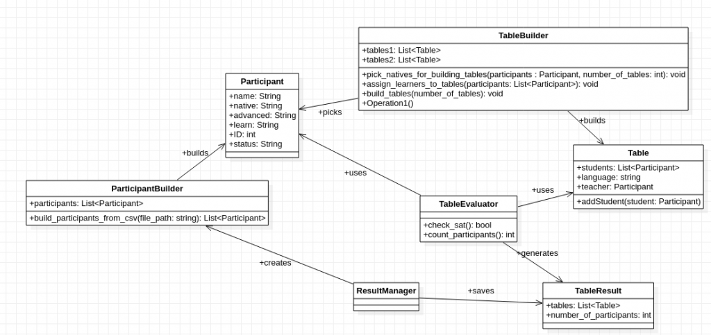
You can find like always the code and a dummy registration file in my GitHub-Repository. In the following picture, you can see the overall UML-diagram of the project. The ResultManager uses the ParticipantBuilder to build participants from the registration file. The TableBuilder builds tables and assigns participants to these tables. The TableEvaluator evaluates the TableBuilder result and saves it. The ResultManager takes care of the best generate result. The random optimization occurs while building the tables and assigning the participants to the tables. The overall process stops after 1000 iterations.
Class diagram of the overall project.
Results
Random Optimization is a method to develop models very fast. This helps us to understand the overall problem much more in detail. When we run this random optimizer on a registration file with 29 participants, it produces an average result with 12 participants (10 times 1000 iterations). This is actually a quite poor result, but now we have got a benchmark for other algorithms, which I will implement as soon I have got more time. So check out my next posts!
The days are getting longer and it is time to prepare for summer again. All the months spent indoors, waiting for the warm weather, eating cookies, and drinking hot chocolate could make you nervous going back to the beach. Imagine a turbocharged workout routine that mixes cardio and strength training and let you train everywhere. Plus, you don’t even need expensive equipment and it’s easily customized to help you to get your best Beach Body ever. Sound too good to be true? It’s not! It’s called circuit training.
Scheveningen, Netherlands
Circuit Training
Circuit training lets you alternate between 4 to 10 exercises that target different muscle groups. The whole idea is to train different muscles all at the same time in a minimum amount of rest. Usually, you train between 15 and 40 minutes. During this time, you will make multiple circuits, with each course containing all exercises. It is a good idea to make 2-3 minute breaks per circuit, 30-90 seconds per exercise, and a 3-5 minute warm-up. The exercises should be arranged so that different muscle groups are trained alternately.
First tries to make a human flag, Germany
To create your perfect circuit training routine you could hire a personal trainer. But let’s be honest: trainers are very expensive. For this task, we will just replace the trainer with an artificial intelligenceagent. The agent will receive our training goals (e.g. a bigger biceps or a six-pack) as input and then tell us our personalized circuit training routine.
Linear Programming
To solve this kind of optimization problem we will use linear programming. Linear programming finds an optimum of a linear function that is subjected to various constraints. You can model a lot of problems as linear functions, finding the perfect circuit training is one of them. To solve our problem we have to do the following steps of the optimization workflow:
Identify the exact problem
Model the problem
Choose a tool to deal with the model
Retrieve the solution
Analysis
One of the first applications of linear programming was in the second world war. But it can also be used for diet optimization, in sports and much more.
In our case, we want to build a circuit training that is as compact as possible and trains all of our muscles. So we want to build a linear function/objective function that describes the total amount of time for the workout. We want to optimize this objective function by modifying the design variables \(x_{i} \in \{0,1\}\).
minimize: \( \sum_{i=1}^{n} t_i \cdot x_{i} \)
The design variable \(x_{i} \in \{0,1\}\) is an exercise and the given coefficents \(t_i\) is the needed time for exercise \(x_i\). \(n\) is the number of exercises.
Each exercise has got its own intensity per muscle group. So pull-ups train for example the biceps, the back and also a little bit abs. But how can we measure the intensity? I define intensity as a value between 0 and 1. 0 means it doesn’t train the specific muscle group at all. 1 means it totally trains the specific muscle group and you don’t need to train this muscle group anymore in the current circle. So I collected a bunch of exercises and defined for each muscle group its intensity and saved it into a CSV-file as a table:
name
shoulders
back
breast
biceps
triceps
abs
butt
butt
legs
squats
0
0
0
0
0
0
1
1
1
pull ups
0.5
1
0
1
0.5
0.5
0
0
0
push ups
0
0
1
0
0.5
0.25
0
0
0
plank
0
0
0
0
0
1
0
0
0
sit-ups
0
0
0
0
0
1
0
0
0
I recommend that you define your own intensities for each exercise. Currently, these intensity values are a little bit relative, if you know a better measurement unit please let me know.
So now we can choose for every circle training how much we want to train at least the specific muscle group. The only thing which is left for our LP-solver is to define these intensities as constraints so that the LP-solver takes the intensities into account. For that reason we create for each muscle group a constraint:
\(y_i \in [0,1]\) is the intensity for exercise \(x_i\).
Code
To solve LP-problems you can use different kinds of LP-solvers. A very nice Open Source LP-solver is PULP. I personally prefer the Gurobi LP-solver, it is a very powerful solver that has got a huge variety of features. If you are in academic you can receive an academic license for free. You can find the full code in my GitHub-Repository.
if __name__ == "__main__":
    # Define your intensities manually
    categories, min_intensity, max_intensity = gp.multidict({
        'shoulders' : [0,GRB.INFINITY],
        'back' : [0,GRB.INFINITY],
        'breast' : [0,GRB.INFINITY],
        'biceps' : [0,GRB.INFINITY],
        'triceps' : [0,GRB.INFINITY],
        'abs' : [0,GRB.INFINITY],
        'butt' : [0.5,0.5],
        'legs' : [2,2]
    })

    # Read exercises and their intensity
    exercises_intensities = build_dict_from_csv_file("exercises.csv", "name")
    # Read exercises and their needed time
    exercises, time = gp.multidict(exercise_and_time_dict(exercises_intensities))
    # Build model
    m = gp.Model("circle_training")
    # Create trainings variables (each exercise is a decision variable)
    training = m.addVars(exercises, vtype=GRB.BINARY, name="training")
    # Objective Function
    m.setObjective(training.prod(time), GRB.MINIMIZE)
    # Constraint:
    # shoulders * push ups + shoulders * biceps + ...
    # others * push ups + ....
    m.addConstrs((gp.quicksum(exercises_intensities[e, c] * training[e] for e in exercises)
        == [min_intensity[c], max_intensity[c]]
        for c in categories), "_"
    )
    # Find Solution
    m.optimize()
    # if there is a solution
    if m.status == GRB.OPTIMAL:
        print("Your training plan:")
        print('\nTime: %g' % m.objVal)
        print('\nTrain:')
        trainingx = m.getAttr('x', training)
        for f in exercises:
            if trainingx[f] > 0:
                print('%s %g' % (f, trainingx[f]))
    else:
        print('No solution')
Are you struggling with what to eat today? Sometimes it is tough to decide, especially if you are hungry and find out there is nothing left in your fridge. I want to show you how it is possible to develop your dish planner and let the computer automatically optimizes your meals according to your daily nutrition intake.
For this program, we use SMT solvers. SMT solvers try to figure out which variable assignment satisfies a given logic formula. If a logic formula is satisfiable, it returns the assigned variables (in our case, your meals). PySMT is a very user-friendly interface for Python developers to encode and solve these kinds of SMT problems. In this post, I give you a small introduction into the field of Satisfiability Modulo Theories by providing you an SMT solver for figuring out what you could eat today.
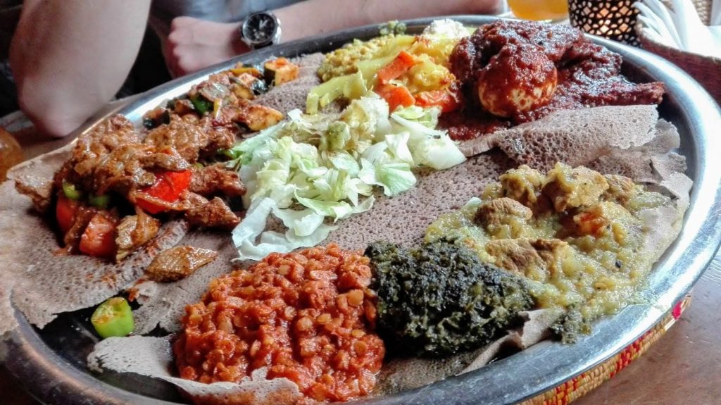
Ethiopian cuisine
Steps
To solve this problem we have to do the following steps:
Create a data set with your favorite dishes (dish name, number of calories, etc. etc.)
Research your daily nutrition intake
Encode a propositional logic formula based on this data set
Let the SMT-solver decide what you should eat
1. Your personalized dish data set
To get your personalized data set, you must figure out how much nutritions are in your dishes. Thanks to the internet there are a variety of websites that provide you with a lot of recipes and the number of nutritions. My favorite ones are:
If you don’t have time to create your data set, I prepared a data set for you. There are many tastes out there, and so I just looked for the most famous food in the world. I ended up with a subset of dishes from CNN travel, and I hope you like it (a lot of them I didn’t know before).
2. Your daily nutrition intake
So how many calories should you eat today? Well, if you’re like me and have got already eaten 3 dishes, much chocolate and haven’t done any sport today, you should probably eat anything. But OK, let’s say the SMT solver should tell you how much you should eat tomorrow. For finding out the exact number of calories you can google for something like “calories calculator” and you may end up on:
(II) \(\sum_{i=1}^{|D|} x_i \cdot d_{i2} \leq (C – \alpha)\\\)
(III) \(\sum_{i=1}^{|D|} x_i = k\)
(IV) \(\bigwedge\limits_{i}^E x_i = 0\)
\( D \) is a set of dishes. \( d_i \in D \) is a tuple \((dish, calories)\) and represents a single dish \(i\).
\(x \in \{ 0, 1 \}\) is an SMT variable that gets automatically assigned by the SMT solver. If \(x_i = 1\), then we will eat this dish the next day. \(k \in \mathbb{N}\) is the number of dishes per day.
\( C \in \mathbb{R} \) is the allowed number of daily calories. \( \alpha \in \mathbb{R} \) is the allowed deviation of \(C\).
\(B\subseteq \mathbb{N}\) is a set of disabled dish indices for the next calculation.
(I) and (II) make sure that our dishes give us the predefined number of calories. (III) makes sure that we get \(k\) dishes per day. (IV) allows us to exclude specific dishes for the next day.
4. Coding
You can find the full code in my GitHub-Repository. This method builds from lines 15 – 53, all the constraints from Section 3. The SMT solving happens at line 55. If a solution is found, it returns the dishes for cooking.
def nutrition_calculator(dishes, number_of_calories, number_of_dishes, disabled_dishes = [], alpha = 100):
    '''
        This method creates a dish plan based on the daily allowed calories
        and the number of dishes.
        Args:
            dishes, pandas data frame. Each row looks like this: (dish name, calories, proteins).
            number_of_calories, the daily number of calories.
            number_of_dishes, the daily number of dishes.
            disabled_dishes, list of row indizes from dishes which are not allowed in the current calculation.
            alpha, the allowed deviation of calories
        Returns:
            row indizes from dishes data frame. These dishes can be eaten today.
    '''
    # Upper and lower calory boundaries
    calories_upper_boundary = Int(int(number_of_calories + alpha))
    calories_lower_boundary = Int(int(number_of_calories - alpha))
    # List of SMT variables
    x = []
    # List of all x_i * d_i2
    x_times_calories = []
    # List of all x_i € {0,1}
    x_zero_or_one = []
    # List of disabled dishes
    x_disabled_sum = []
    for index, row in dishes.iterrows():
        x.append(Symbol('x' + str(index), INT))
        # x_i * d_i2
        x_times_calories.append(Times(x[-1], Int(row.calories)))
        # x_i € {0,1}
        x_zero_or_one.append(Or(Equals(x[-1], Int(0)), Equals(x[-1], Int(1))))
        # Disable potential dishes
        if index in disabled_dishes:
            x_disabled_sum.append(x[-1])
    x_times_calories_sum = Plus(x_times_calories)
    x_sum = Plus(x)
    if len(x_disabled_sum) == 0:
        x_disabled_sum = Int(0)
    else:
        x_disabled_sum = Plus(x_disabled_sum)
    formula = And(
        [
            # Makes sure that our calories are above the lower boundary
            GE(x_times_calories_sum, calories_lower_boundary),
            # Makes sure that our calories are below the upper boundary
            LE(x_times_calories_sum, calories_upper_boundary),
            # Makes sure that we get number_of_dishes dishes per day
            Equals(x_sum, Int(int(number_of_dishes))),
            # Makes sure that we don't use the disabled dishes
            Equals(x_disabled_sum, Int(0)),
            # Makes sure that each dish is maximal used once
            And(x_zero_or_one)
        ]
    )
    # SMT solving
    model = get_model(formula)
    # Get indizes
    if model:
        result_indizes = []
        for i in range(len(x)):
            if(model.get_py_value(x[i]) == 1):
                result_indizes.append(i)
        return result_indizes
    else:
        return None
Extensions & More
We can easily add two further constraints to support e.g. proteins in our encoding:
\( P \in \mathbb{R} \) is the allowed number of proteins. \( \beta \in \mathbb{R} \) is the allowed deviation of \(P\). Don’t forget to update our set of dishes \(D\) and extend our tuple \(d_i\) to \((dish, calories, proteins)\).
If you want to learn more about SMT solving, check out the following links: